Some Known Incorrect Statements About Interview Questions

By pushing ctrl+shift+center, this will certainly compute and return value from numerous varieties, instead of just private cells added to or increased by each other. Calculating the amount, item, or ratio of individual cells is very easy-- just use the =AMOUNT formula and also enter the cells, values, or series of cells you intend to perform that arithmetic on.

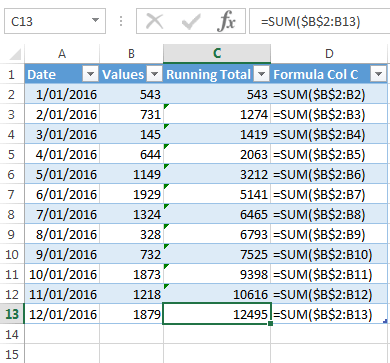
If you're wanting to find overall sales revenue from several marketed systems, as an example, the variety formula in Excel is ideal for you. Here's just how you 'd do it: To begin using the selection formula, kind "=SUM," and in parentheses, get in the very first of 2 (or three, or 4) varieties of cells you wish to increase together.

This means reproduction. Following this asterisk, enter your second array of cells. You'll be multiplying this second series of cells by the first. Your development in this formula should now resemble this: =AMOUNT(C 2: C 5 * D 2:D 5) Ready to push Get in? Not so quick ... Since this formula is so difficult, Excel reserves a different key-board command for selections.

This will certainly recognize your formula as a range, covering your formula in brace personalities and also successfully returning your product of both varieties combined. In income calculations, this can lower your effort and time considerably. See the final formula in the screenshot above. The MATTER formula in Excel is represented =COUNT(Begin Cell: End Cell).

For instance, if there are eight cells with gotten in values in between A 1 and also A 10, =COUNT(A 1: A 10) will return a worth of 8. The MATTER formula in Excel is particularly helpful for large spread sheets, in which you desire to see exactly how numerous cells contain actual access. Do not be tricked: This formula will not do any kind of math on the values of the cells themselves.

About Interview Questions

Making use of the formula in vibrant over, you can quickly run a count of active cells in your spread sheet. The result will certainly look a little something like this: To perform the ordinary formula in Excel, get in the worths, cells, or array of cells of which you're computing the standard in the format, =AVERAGE(number 1, number 2, etc.) or =STANDARD(Start Worth: End Worth).

Discovering the average of a series of cells in Excel keeps you from needing to locate private sums and also then performing a different department equation on your total. Making use of =STANDARD as your preliminary message entry, you can let Excel do all the help you. For referral, the average of a team of numbers is equal to the sum of those numbers, divided by the variety of things because team.

This will certainly return the sum of the worths within a preferred array of cells that all meet one criterion. For instance, =SUMIF(C 3: C 12,"> 70,000") would return the sum of worths between cells C 3 and also C 12 from just the cells that are better than 70,000. Allow's say you intend to identify the profit you generated from a listing of leads that are related to details location codes, or calculate the amount of particular employees' wages-- yet only if they drop above a certain quantity.

With the SUMIF feature, it does not have to be-- you can conveniently add up the amount of cells that satisfy particular requirements, like in the salary example above. The formula: =SUMIF(array, standards, [sum_range] Range: The variety that is being tested using your standards. Standards: The standards that determine which cells in Criteria_range 1 will certainly be combined [Sum_range]: An optional array of cells you're mosting likely to accumulate along with the very first Array went into.

In the instance below, we wished to determine the sum of the wages that were above $70,000. The SUMIF function accumulated the buck amounts that exceeded that number in the cells C 3 through C 12, with the formula =SUMIF(C 3: C 12,"> 70,000"). The TRIM formula in Excel is denoted =TRIM(message).

The 45-Second Trick For Excel Shortcuts

For instance, if A 2 includes the name" Steve Peterson" with undesirable rooms before the very first name, =TRIM(A 2) would return "Steve Peterson" with no spaces in a brand-new cell. Email as well as file sharing are terrific tools in today's work environment. That is, until one of your coworkers sends you a worksheet with some truly fashionable spacing.

As opposed to meticulously removing as well as adding areas as required, you can tidy up any uneven spacing making use of the TRIM function, which is used to get rid of extra spaces from data (other than for single spaces between words). The formula: =TRIM(text). Text: The message or cell where you desire to remove areas.

To do so, we got in =TRIM("A 2") into the Formula Bar, and also reproduced this for every name below it in a brand-new column beside the column with unwanted rooms. Below are some other Excel solutions you might locate useful as your information administration requires expand. Let's say you have a line of message within a cell that you wish to damage down into a couple of various sectors.

Function: Made use of to draw out the first X numbers or characters in a cell. The formula: =LEFT(message, number_of_characters) Text: The string that you wish to remove from. Number_of_characters: The number of characters that you desire to extract starting from the left-most personality. In the instance below, we went into =LEFT(A 2,4) into cell B 2, as well as duplicated it right into B 3: B 6.

Objective: Made use of to extract characters or numbers between based upon setting. The formula: =MID(message, start_position, number_of_characters) Text: The string that you want to extract from. Start_position: The placement in the string that you intend to start removing from. As an example, the very first placement in the string is 1.

Sumif Excel - The Facts

In this instance, we went into =MID(A 2,5,2) into cell B 2, and also duplicated it right into B 3: B 6. That enabled us to remove the two numbers starting in the fifth setting of the code. Objective: Made use of to draw out the last X numbers or characters in a cell. The formula: =RIGHT(text, number_of_characters) Text: The string that you desire to extract from.

excel formulas español excel formulas khmer excel formulas tutorials pdf